Propositional Equation Reasoning Systems
- Note. The MathJax parser is not rendering this page properly.
Until it can be fixed please see the InterSciWiki version.
Author: Jon Awbrey
This article develops elementary facts about a family of formal calculi described as propositional equation reasoning systems (PERS). This work follows on the alpha graphs that Charles Sanders Peirce devised as a graphical syntax for propositional calculus and also on the calculus of indications that George Spencer Brown presented in his Laws of Form.
Formal development
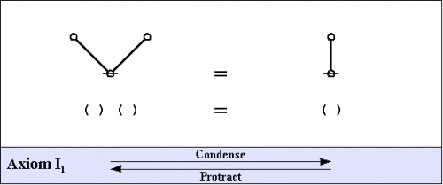
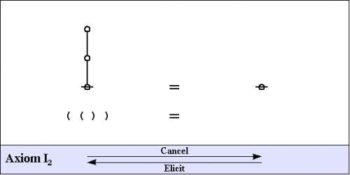
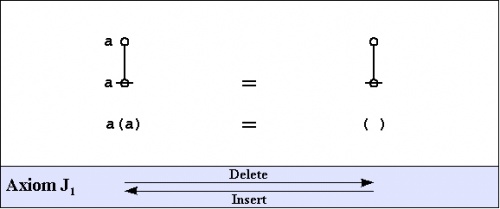
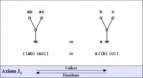
The first order of business is to give the exact forms of the axioms that we use, devolving from Peirce's “Logical Graphs” via Spencer-Brown's Laws of Form (LOF). In formal proofs, we use a variation of the annotation scheme from LOF to mark each step of the proof according to which axiom, or initial, is being invoked to justify the corresponding step of syntactic transformation, whether it applies to graphs or to strings.
Axioms
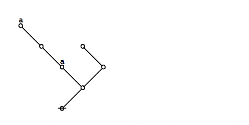
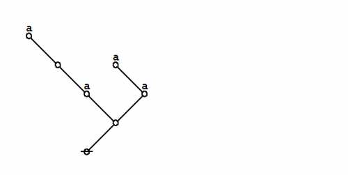
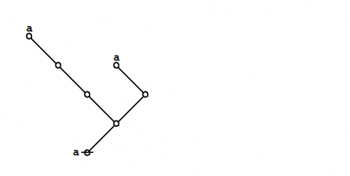
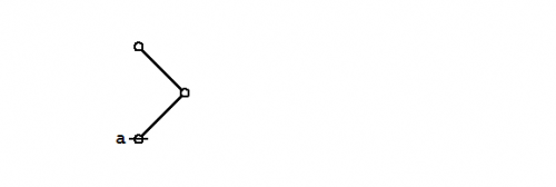
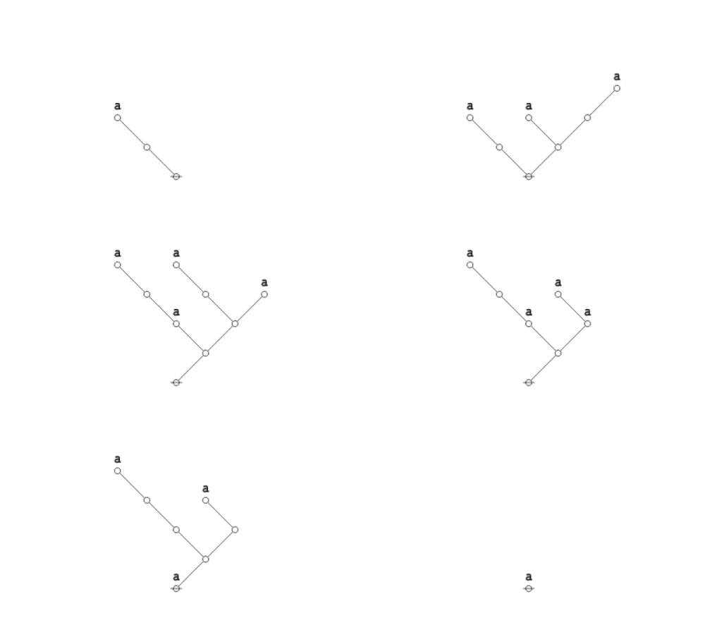
The axioms are just four in number, divided into the arithmetic initials, \(I_1\!\) and \(I_2,\!\) and the algebraic initials, \(J_1\!\) and \(J_2.\!\)
 |
(1) |
 |
(2) |
 |
(3) |
 |
(4) |
One way of assigning logical meaning to the initial equations is known as the entitative interpretation \((\mathrm{En}).\!\) Under \(\mathrm{En},\!\) the axioms read as follows:
|
\(\begin{matrix} I_1 & : & \mathrm{true} ~\mathrm{or}~ \mathrm{true} & = & \mathrm{true} \\ I_2 & : & \mathrm{not}~ \mathrm{true} & = & \mathrm{false} \\ J_1 & : & a ~\mathrm{or}~ \mathrm{not}~ a & = & \mathrm{true} \\ J_2 & : & (a ~\mathrm{or}~ b) ~\mathrm{and}~ (a ~\mathrm{or}~ c) & = & a ~\mathrm{or}~ (b ~\mathrm{and}~ c) \end{matrix}\) |
Another way of assigning logical meaning to the initial equations is known as the existential interpretation \((\mathrm{Ex}).\!\) Under \(\mathrm{Ex},\!\) the axioms read as follows:
|
\(\begin{matrix} I_1 & : & \mathrm{false} ~\mathrm{and}~ \mathrm{false} & = & \mathrm{false} \\ I_2 & : & \mathrm{not}~ \mathrm{false} & = & \mathrm{true} \\ J_1 & : & a ~\mathrm{and}~ \mathrm{not}~ a & = & \mathrm{false} \\ J_2 & : & (a ~\mathrm{and}~ b) ~\mathrm{or}~ (a ~\mathrm{and}~ c) & = & a ~\mathrm{and}~ (b ~\mathrm{or}~ c) \end{matrix}\) |
All of the axioms in this set have the form of equations. This means that all of the inference licensed by them are reversible. The proof annotation scheme employed below makes use of a double bar ═════ to mark this fact, but it will often be left to the reader to decide which of the two possible ways of applying the axiom is the one that is called for in a particular case.
Peirce introduced these formal equations at a level of abstraction that is one step higher than their customary interpretations as propositional calculi, which two readings he called the Entitative and the Existential interpretations, here referred to as \(\mathrm{En}\!\) and \(\mathrm{Ex},\!\) respectively. The early CSP, as in his essay on “Qualitative Logic”, and also GSB, emphasized the \(\mathrm{En}\!\) interpretation, while the later CSP developed mostly the \(\mathrm{Ex}\!\) interpretation.
Frequently used theorems
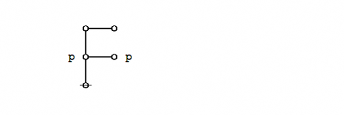
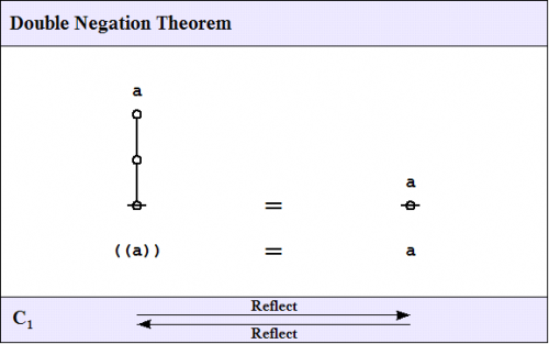
C1. Double negation
The first theorem goes under the names of Consequence 1 \((C_1),\!\) the double negation theorem (DNT), or Reflection.
 |
(5) |
The proof that follows is adapted from the one that was given by George Spencer Brown in his book Laws of Form (LOF) and credited to two of his students, John Dawes and D.A. Utting.
|
(6) |
The steps of this proof are replayed in the following animation.
|
(7) |
C2. Generation theorem
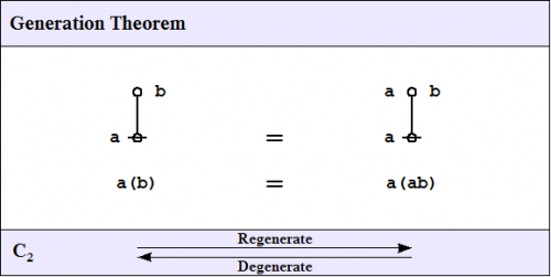
One theorem of frequent use goes under the nickname of the weed and seed theorem (WAST). The proof is just an exercise in mathematical induction, once a suitable basis is laid down, and it will be left as an exercise for the reader. What the WAST says is that a label can be freely distributed or freely erased anywhere in a subtree whose root is labeled with that label. The second in our list of frequently used theorems is in fact the base case of this weed and seed theorem. In LOF, it goes by the names of Consequence 2 \((C_2)\!\) or Generation.
 |
(8) |
Here is a proof of the Generation Theorem.
|
(9) |
The steps of this proof are replayed in the following animation.
|
(10) |
C3. Dominant form theorem
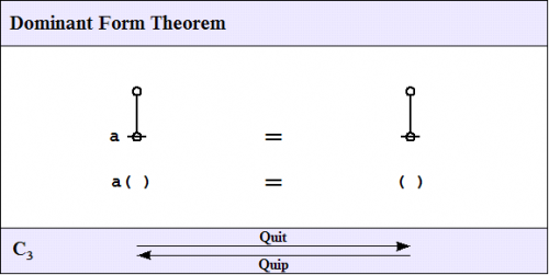
The third of the frequently used theorems of service to this survey is one that Spencer-Brown annotates as Consequence 3 \((C_3)\!\) or Integration. A better mnemonic might be dominance and recession theorem (DART), but perhaps the brevity of dominant form theorem (DFT) is sufficient reminder of its double-edged role in proofs.
 |
(11) |
Here is a proof of the Dominant Form Theorem.
|
(12) |
The following animation provides an instant re*play.
|
(13) |
Exemplary proofs
Based on the axioms given at the outest, and aided by the theorems recorded so far, it is possible to prove a multitude of much more complex theorems. A couple of all-time favorites are given next.
Peirce's law
- Main article : Peirce's law
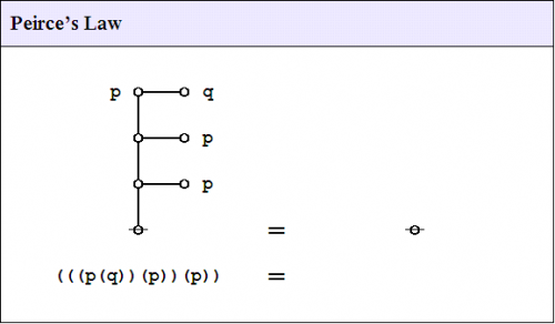
Peirce's law is commonly written in the following form:
| \(((p \Rightarrow q) \Rightarrow p) \Rightarrow p\!\) |
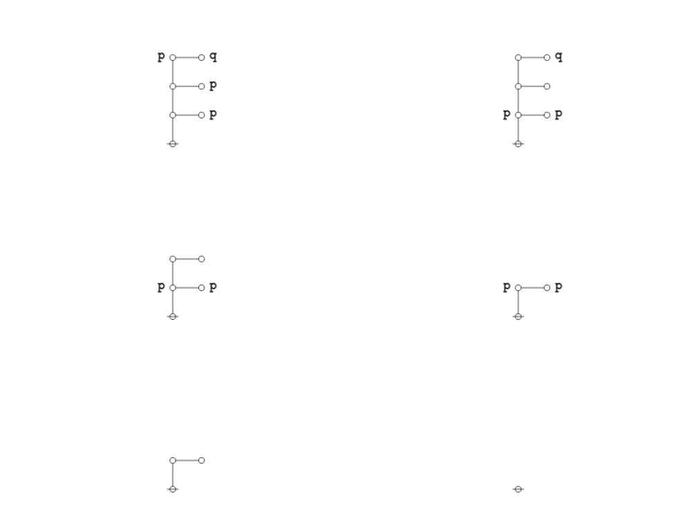
The existential graph representation of Peirce's law is shown below.
 |
(14) |
A graphical proof of Peirce's law is shown next.
|
(15) |
The following animation replays the steps of the proof.
|
(16) |
Praeclarum theorema
An illustrious example of a propositional theorem is the praeclarum theorema, the admirable, shining, or splendid theorem of Leibniz.
|
If a is b and d is c, then ad will be bc. This is a fine theorem, which is proved in this way: a is b, therefore ad is bd (by what precedes), d is c, therefore bd is bc (again by what precedes), ad is bd, and bd is bc, therefore ad is bc. Q.E.D. (Leibniz, Logical Papers, p. 41). |
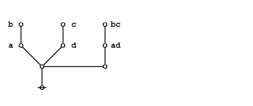
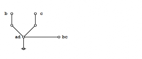
Under the existential interpretation, the praeclarum theorema is represented by means of the following logical graph.
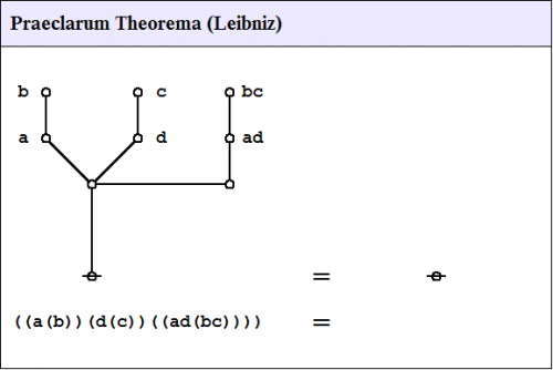 |
(17) |
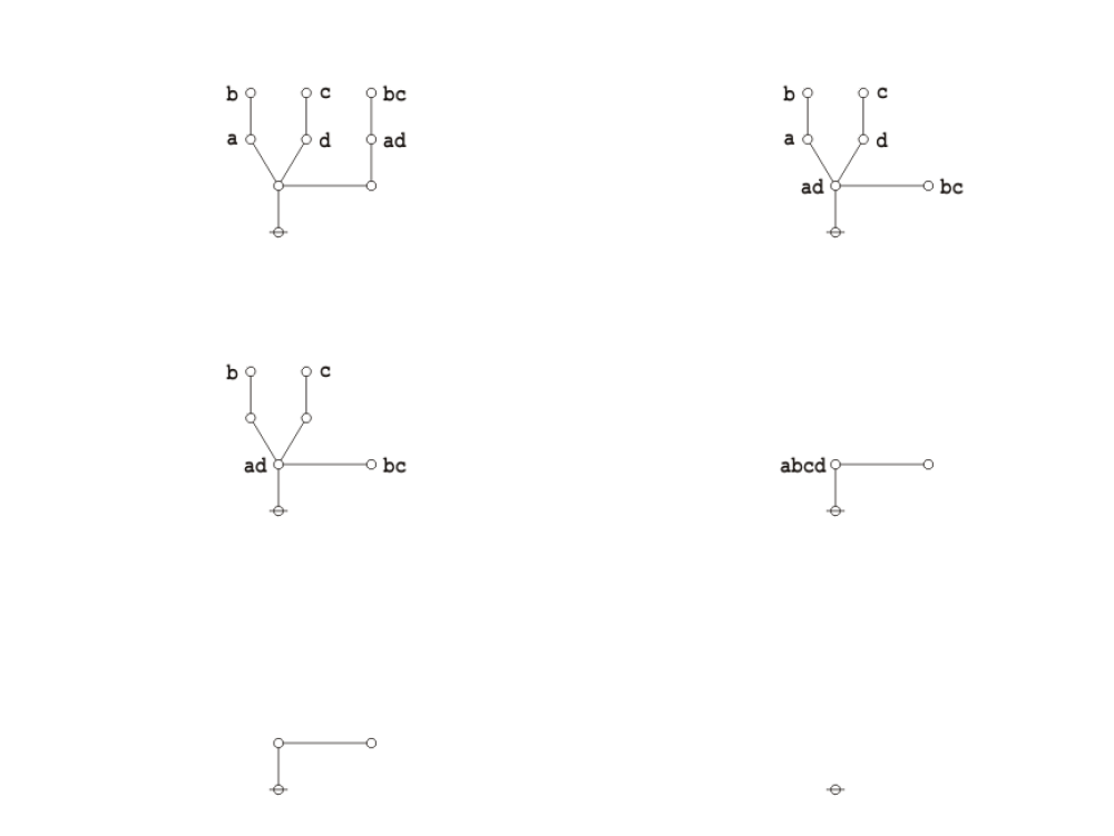
And here's a neat proof of that nice theorem.
|
(18) |
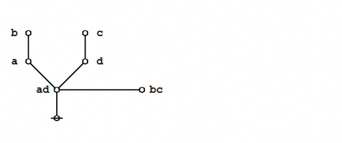
The steps of the proof are replayed in the following animation.
|
(19) |
Two-thirds majority function
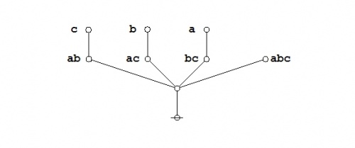
Consider the following equation in boolean algebra, posted as a problem for proof at MathOverFlow.
|
\(\begin{matrix} a b \bar{c} + a \bar{b} c + \bar{a} b c + a b c \\[6pt] \iff \\[6pt] a b + a c + b c \end{matrix}\) |
(20) |
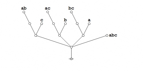
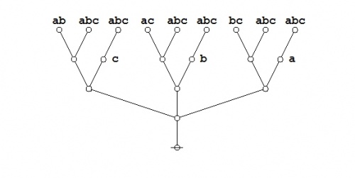
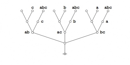
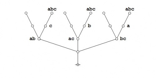
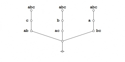
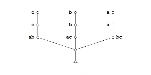
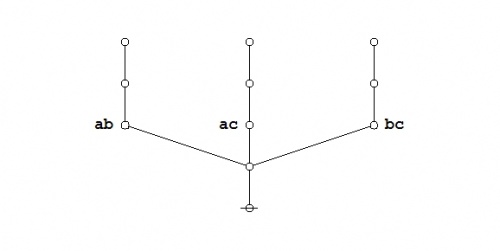
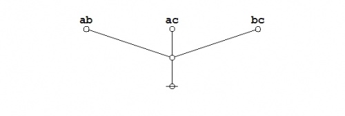
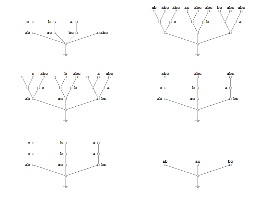
The required equation can be proven in the medium of logical graphs as shown in the following Figure.
|
(21) |
Here's an animated recap of the graphical transformations that occur in the above proof:
|
(22) |
Formal extension : Cactus calculus
Let us now extend the CSP–GSB calculus in the following way:

