|
\(\begin{array}{c|c}
t & x \'"`UNIQ-MathJax1-QINU`"' in other words'"`UNIQ-MathJax2-QINU`"'
=='"`UNIQ--h-10--QINU`"'Notions of Approximation==
{| cellpadding="2" cellspacing="2" width="100%"
| width="60%" |
| width="40%" |
for equalities are so weighed<br>
that curiosity in neither can<br>
make choice of either's moiety.
|-
| height="50px" |
| valign="top" | — ''King Lear'', Sc.1.5–7 (Quarto)
|-
|
|
for qualities are so weighed<br>
that curiosity in neither can<br>
make choice of either's moiety.<br>
|-
| height="50px" |
| valign="top" | — ''King Lear'', 1.1.5–6 (Folio)
|}
Justifying a notion of approximation is a little more involved in general, and especially in these discrete logical spaces, than it would be expedient for people in a hurry to tangle with right now. I will just say that there are ''naive'' or ''obvious'' notions and there are ''sophisticated'' or ''subtle'' notions that we might choose among. The later would engage us in trying to construct proper logical analogues of Lie derivatives, and so let's save that for when we have become subtle or sophisticated or both. Against or toward that day, as you wish, let's begin with an option in plain view.
Figure 1.4 illustrates one way of ranging over the cells of the underlying universe \(U^\bullet = [u, v]\!\) and selecting at each cell the linear proposition in \(\mathrm{d}U^\bullet = [\mathrm{d}u, \mathrm{d}v]\!\) that best approximates the patch of the difference map \({\mathrm{D}f}\!\) that is located there, yielding the following formula for the differential \(\mathrm{d}f.\!\)
|
\(\begin{array}{*{11}{c}}
\mathrm{d}f
& = & \mathrm{d}\texttt{((} u \texttt{)(} v \texttt{))}
& = & uv \cdot 0
& + & u \texttt{(} v \texttt{)} \cdot \mathrm{d}u
& + & \texttt{(} u \texttt{)} v \cdot \mathrm{d}v
& + & \texttt{(} u \texttt{)(} v \texttt{)} \cdot \texttt{(} \mathrm{d}u \texttt{,~} \mathrm{d}v \texttt{)}
\end{array}\)
|
o---------------------------------------o
|                                       |
|                   o                   |
|                  / \                  |
|                 /   \                 |
|                /     \                |
|               o       o               |
|              / \     / \              |
|             /   \   /   \             |
|            /     \ /     \            |
|           o       o       o           |
|          / \     / \     / \          |
|         /   \   /   \   /   \         |
|        /     \ /     \ /     \        |
|       o       o       o       o       |
|      / \     /%\     /%\     / \      |
|     /   \   /%%%\   /%%%\   /   \     |
|    /     \ /%%%%%\ /%%%%%\ /     \    |
|   o       o%%%%%%%o%%%%%%%o       o   |
|   |\     /%\%%%%%/ \%%%%%/%\     /|   |
|   | \   /%%%\%%%/   \%%%/%%%\   / |   |
|   |  \ /%%%%%\%/     \%/%%%%%\ /  |   |
|   |   o%%%%%%%o       o%%%%%%%o   |   |
|   |   |\%%%%%/%\     /%\%%%%%/|   |   |
|   |   | \%%%/%%%\   /%%%\%%%/ |   |   |
|   | u |  \%/%%%%%\ /%%%%%\%/  | v |   |
|   o---+---o%%%%%%%o%%%%%%%o---+---o   |
|       |    \%%%%%/ \%%%%%/    |       |
|       |     \%%%/   \%%%/     |       |
|       | du   \%/     \%/   dv |       |
|       o-------o       o-------o       |
|                \     /                |
|                 \   /                 |
|                  \ /                  |
|                   o                   |
|                                       |
o---------------------------------------o
Figure 1.4.  df = linear approx to Df
|
Figure 2.4 illustrates one way of ranging over the cells of the underlying universe \(U^\bullet = [u, v]\!\) and selecting at each cell the linear proposition in \(\mathrm{d}U^\bullet = [du, dv]\!\) that best approximates the patch of the difference map \(\mathrm{D}g\!\) that is located there, yielding the following formula for the differential \(\mathrm{d}g.\!\)
|
\(\begin{array}{*{11}{c}}
\mathrm{d}g
& = & \mathrm{d}\texttt{((} u \texttt{,} v \texttt{))}
& = & uv \cdot \texttt{(} \mathrm{d}u \texttt{,} \mathrm{d}v \texttt{)}
& + & u \texttt{(} v \texttt{)} \cdot \texttt{(} \mathrm{d}u \texttt{,} \mathrm{d}v \texttt{)}
& + & \texttt{(} u \texttt{)} v \cdot \texttt{(} \mathrm{d}u \texttt{,} \mathrm{d}v \texttt{)}
& + & \texttt{(} u \texttt{)(} v \texttt{)} \cdot \texttt{(} \mathrm{d}u \texttt{,} \mathrm{d}v \texttt{)}
\end{array}\)
|
o---------------------------------------o
|                                       |
|                   o                   |
|                  / \                  |
|                 /   \                 |
|                /     \                |
|               o       o               |
|              /%\     /%\              |
|             /%%%\   /%%%\             |
|            /%%%%%\ /%%%%%\            |
|           o%%%%%%%o%%%%%%%o           |
|          /%\%%%%%/ \%%%%%/%\          |
|         /%%%\%%%/   \%%%/%%%\         |
|        /%%%%%\%/     \%/%%%%%\        |
|       o%%%%%%%o       o%%%%%%%o       |
|      / \%%%%%/ \     / \%%%%%/ \      |
|     /   \%%%/   \   /   \%%%/   \     |
|    /     \%/     \ /     \%/     \    |
|   o       o       o       o       o   |
|   |\     /%\     / \     /%\     /|   |
|   | \   /%%%\   /   \   /%%%\   / |   |
|   |  \ /%%%%%\ /     \ /%%%%%\ /  |   |
|   |   o%%%%%%%o       o%%%%%%%o   |   |
|   |   |\%%%%%/%\     /%\%%%%%/|   |   |
|   |   | \%%%/%%%\   /%%%\%%%/ |   |   |
|   | u |  \%/%%%%%\ /%%%%%\%/  | v |   |
|   o---+---o%%%%%%%o%%%%%%%o---+---o   |
|       |    \%%%%%/ \%%%%%/    |       |
|       |     \%%%/   \%%%/     |       |
|       | du   \%/     \%/   dv |       |
|       o-------o       o-------o       |
|                \     /                |
|                 \   /                 |
|                  \ /                  |
|                   o                   |
|                                       |
o---------------------------------------o
Figure 2.4.  dg = linear approx to Dg
|
Well, \(g,\!\) that was easy, seeing as how \(\mathrm{D}g\!\) is already linear at each locus, \(\mathrm{d}g = \mathrm{D}g.\!\)
Analytic Series
We have been conducting the differential analysis of the logical transformation \(F : [u, v] \mapsto [u, v]\!\) defined as \(F : (u, v) \mapsto ( ~ \texttt{((} u \texttt{)(} v \texttt{))} ~,~ \texttt{((} u \texttt{,~} v \texttt{))} ~ ),\!\) and this means starting with the extended transformation \(\mathrm{E}F : [u, v, \mathrm{d}u, \mathrm{d}v] \to [u, v, \mathrm{d}u, \mathrm{d}v]\!\) and breaking it into an analytic series, \(\mathrm{E}F = F + \mathrm{d}F + \mathrm{d}^2 F + \ldots,\!\) and so on until there is nothing left to analyze any further.
As a general rule, one proceeds by way of the following stages:
|
\(\begin{array}{*{6}{l}}
1. & \mathrm{E}F
& = & \mathrm{d}^0 F
& + & \mathrm{r}^0 F
\\
2. & \mathrm{r}^0 F
& = & \mathrm{d}^1 F
& + & \mathrm{r}^1 F
\\
3. & \mathrm{r}^1 F
& = & \mathrm{d}^2 F
& + & \mathrm{r}^2 F
\\
4. & \ldots
\end{array}\)
|
In our analysis of the transformation \(F,\!\) we carried out Step 1 in the more familiar form \(\mathrm{E}F = F + \mathrm{D}F\!\) and we have just reached Step 2 in the form \(\mathrm{D}F = \mathrm{d}F + \mathrm{r}F,\!\) where \(\mathrm{r}F\!\) is the residual term that remains for us to examine next.
Note. I'm am trying to give quick overview here, and this forces me to omit many picky details. The picky reader may wish to consult the more detailed presentation of this material at the following locations:
-
Let's push on with the analysis of the transformation:
|
\(\begin{matrix}
F & : & (u, v) & \mapsto & (f(u, v), g(u, v))
& = & ( ~ \texttt{((} u \texttt{)(} v \texttt{))} ~,~ \texttt{((} u \texttt{,~} v \texttt{))} ~)
\end{matrix}\)
|
For ease of comparison and computation, I will collect the Figures that we need for the remainder of the work together on one page.
Computation Summary for Logical Disjunction
Figure 1.1 shows the expansion of \(f = \texttt{((} u \texttt{)(} v \texttt{))}\!\) over \([u, v]\!\) to produce the expression:
|
\(\begin{matrix}
uv & + & u \texttt{(} v \texttt{)} & + & \texttt{(} u \texttt{)} v
\end{matrix}\)
|
Figure 1.2 shows the expansion of \(\mathrm{E}f = \texttt{((} u + \mathrm{d}u \texttt{)(} v + \mathrm{d}v \texttt{))}\!\) over \([u, v]\!\) to produce the expression:
|
\(\begin{matrix}
uv \cdot \texttt{(} \mathrm{d}u ~ \mathrm{d}v \texttt{)} & + &
u \texttt{(} v \texttt{)} \cdot \texttt{(} \mathrm{d}u \texttt{(} \mathrm{d}v \texttt{))} & + &
\texttt{(} u \texttt{)} v \cdot \texttt{((} \mathrm{d}u \texttt{)} \mathrm{d}v \texttt{)} & + &
\texttt{(} u \texttt{)(} v \texttt{)} \cdot \texttt{((} \mathrm{d}u \texttt{)(} \mathrm{d}v \texttt{))}
\end{matrix}\)
|
In general, \(\mathrm{E}f\!\) tells you what you would have to do, from wherever you are in the universe \([u, v],\!\) if you want to end up in a place where \(f\!\) is true. In this case, where the prevailing proposition \(f\!\) is \(\texttt{((} u \texttt{)(} v \texttt{))},\!\) the indication \(uv \cdot \texttt{(} \mathrm{d}u ~ \mathrm{d}v \texttt{)}\!\) of \(\mathrm{E}f\!\) tells you this: If \(u\!\) and \(v\!\) are both true where you are, then just don't change both \(u\!\) and \(v\!\) at once, and you will end up in a place where \(\texttt{((} u \texttt{)(} v \texttt{))}\!\) is true.
Figure 1.3 shows the expansion of \(\mathrm{D}f\) over \([u, v]\!\) to produce the expression:
|
\(\begin{matrix}
uv \cdot \mathrm{d}u ~ \mathrm{d}v & + &
u \texttt{(} v \texttt{)} \cdot \mathrm{d}u \texttt{(} \mathrm{d}v \texttt{)} & + &
\texttt{(} u \texttt{)} v \cdot \texttt{(} \mathrm{d}u \texttt{)} \mathrm{d}v & + &
\texttt{(} u \texttt{)(} v \texttt{)} \cdot \texttt{((} \mathrm{d}u \texttt{)(} \mathrm{d}v \texttt{))}
\end{matrix}\)
|
In general, \({\mathrm{D}f}\!\) tells you what you would have to do, from wherever you are in the universe \([u, v],\!\) if you want to bring about a change in the value of \(f,\!\) that is, if you want to get to a place where the value of \(f\!\) is different from what it is where you are. In the present case, where the reigning proposition \(f\!\) is \(\texttt{((} u \texttt{)(} v \texttt{))},\!\) the term \(uv \cdot \mathrm{d}u ~ \mathrm{d}v\!\) of \({\mathrm{D}f}\!\) tells you this: If \(u\!\) and \(v\!\) are both true where you are, then you would have to change both \(u\!\) and \(v\!\) in order to reach a place where the value of \(f\!\) is different from what it is where you are.
Figure 1.4 approximates \({\mathrm{D}f}\!\) by the linear form \(\mathrm{d}f\!\) that expands over \([u, v]\!\) as follows:
|
\(\begin{matrix}
\mathrm{d}f
& = & uv \cdot 0
& + & u \texttt{(} v \texttt{)} \cdot \mathrm{d}u
& + & \texttt{(} u \texttt{)} v \cdot \mathrm{d}v
& + & \texttt{(} u \texttt{)(} v \texttt{)} \cdot \texttt{(} \mathrm{d}u \texttt{,~} \mathrm{d}v \texttt{)}
\'"`UNIQ-MathJax3-QINU`"' Another way to convey the same information is by means of the extended proposition'"`UNIQ-MathJax4-QINU`"'
{| align="center" cellpadding="8" style="text-align:center"
| \(\text{Orbit 2}\!\)
|
|
\(\begin{array}{c|cc|cc|cc|}
t & u & v & \mathrm{d}u & \mathrm{d}v & \mathrm{d}^2 u & \mathrm{d}^2 v \\[8pt]
0 & 0 & 0 & 0 & 1 & 1 & 0 \\
1 & 0 & 1 & 1 & 1 & 1 & 1 \\
2 & 1 & 0 & 0 & 0 & 0 & 0 \\
3 & {}^\shortparallel & {}^\shortparallel & {}^\shortparallel & {}^\shortparallel & {}^\shortparallel & {}^\shortparallel
\end{array}\)
|
A more fine combing of the second Table brings to mind a rule that partly covers the remaining cases, that is, \(\mathrm{d}u = v, ~ \mathrm{d}v = \texttt{(} u \texttt{)}.\!\) This much information about Orbit 2 is also encapsulated by the extended proposition \(\texttt{(} uv \texttt{)((} \mathrm{d}u \texttt{,} v \texttt{))(} \mathrm{d}v, u \texttt{)},\!\) which says that \(u\!\) and \(v\!\) are not both true at the same time, while \(\mathrm{d}u\!\) is equal in value to \(v\!\) and \(\mathrm{d}v\!\) is opposite in value to \(u.\!\)
Turing Machine Example
☞ See Theme One Program for documentation of the cactus graph syntax and the propositional modeling program used below.
By way of providing a simple illustration of Cook's Theorem, namely, that “Propositional Satisfiability is NP-Complete”, I will describe one way to translate finite approximations of turing machines into propositional expressions, using the cactus language syntax for propositional calculus that I will describe in more detail as we proceed.
- \(\mathrm{Stilt}(k) =\!\)
- Space and time limited turing machine,
- with \(k\!\) units of space and \(k\!\) units of time.
- \(\mathrm{Stunt}(k) =\!\)
- Space and time limited turing machine,
- for computing the parity of a bit string, with number of tape cells of input equal to \(k.\!\)
I will follow the pattern of discussion in Herbert Wilf (1986), Algorithms and Complexity, pp. 188–201, but translate his logical formalism into cactus language, which is more efficient in regard to the number of propositional clauses that are required.
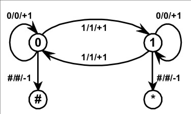
A turing machine for computing the parity of a bit string is described by means of the following Figure and Table.
|
| \(\text{Figure 3.} ~~ \text{Parity Machine}\!\)
|
Table 4.  Parity Machine
o-------o--------o-------------o---------o------------o
| State | Symbol | Next Symbol | Ratchet | Next State |
|   Q   |   S    |     S'      |   dR    |     Q'     |
o-------o--------o-------------o---------o------------o
|   0   |   0    |     0       |   +1    |     0      |
|   0   |   1    |     1       |   +1    |     1      |
|   0   |   #    |     #       |   -1    |     #      |
|   1   |   0    |     0       |   +1    |     1      |
|   1   |   1    |     1       |   +1    |     0      |
|   1   |   #    |     #       |   -1    |     *      |
o-------o--------o-------------o---------o------------o
|
The TM has a finite automaton (FA) as one component. Let us refer to this particular FA by the name of \(\mathrm{M}.\)
The tape head (that is, the read unit) will be called \(\mathrm{H}.\) The registers are also called tape cells or tape squares.
Finite Approximations
To see how each finite approximation to a given turing machine can be given a purely propositional description, one fixes the parameter \(k\!\) and limits the rest of the discussion to describing \(\mathrm{Stilt}(k),\!\) which is not really a full-fledged TM anymore but just a finite automaton in disguise.
In this example, for the sake of a minimal illustration, we choose \(k = 2,\!\) and discuss \(\mathrm{Stunt}(2).\) Since the zeroth tape cell and the last tape cell are both occupied by the character \(^{\backprime\backprime}\texttt{\#}^{\prime\prime}\) that is used for both the beginning of file \((\mathrm{bof})\) and the end of file \((\mathrm{eof})\) markers, this allows for only one digit of significant computation.
To translate \(\mathrm{Stunt}(2)\) into propositional form we use the following collection of basic propositions, boolean variables, or logical features, depending on what one prefers to call them:
The basic propositions for describing the present state function \(\mathrm{QF} : P \to Q\) are these:
|
\(\begin{matrix}
\texttt{p0\_q\#}, & \texttt{p0\_q*}, & \texttt{p0\_q0}, & \texttt{p0\_q1},
\\[6pt]
\texttt{p1\_q\#}, & \texttt{p1\_q*}, & \texttt{p1\_q0}, & \texttt{p1\_q1},
\\[6pt]
\texttt{p2\_q\#}, & \texttt{p2\_q*}, & \texttt{p2\_q0}, & \texttt{p2\_q1},
\\[6pt]
\texttt{p3\_q\#}, & \texttt{p3\_q*}, & \texttt{p3\_q0}, & \texttt{p3\_q1}.
\end{matrix}\)
|
The proposition of the form \(\texttt{pi\_qj}\) says:
| At the point-in-time \(p_i,\!\) the finite state machine \(\mathrm{M}\) is in the state \(q_j.\!\)
|
The basic propositions for describing the present register function \(\mathrm{RF} : P \to R\) are these:
|
\(\begin{matrix}
\texttt{p0\_r0}, & \texttt{p0\_r1}, & \texttt{p0\_r2}, & \texttt{p0\_r3},
\\[6pt]
\texttt{p1\_r0}, & \texttt{p1\_r1}, & \texttt{p1\_r2}, & \texttt{p1\_r3},
\\[6pt]
\texttt{p2\_r0}, & \texttt{p2\_r1}, & \texttt{p2\_r2}, & \texttt{p2\_r3},
\\[6pt]
\texttt{p3\_r0}, & \texttt{p3\_r1}, & \texttt{p3\_r2}, & \texttt{p3\_r3}.
\end{matrix}\)
|
The proposition of the form \(\texttt{pi\_rj}\) says:
| At the point-in-time \(p_i,\!\) the tape head \(\mathrm{H}\) is on the tape cell \(r_j.\!\)
|
The basic propositions for describing the present symbol function \(\mathrm{SF} : P \to (R \to S)\) are these:
|
\(\begin{matrix}
\texttt{p0\_r0\_s\#}, & \texttt{p0\_r0\_s*}, & \texttt{p0\_r0\_s0}, & \texttt{p0\_r0\_s1},
\\[4pt]
\texttt{p0\_r1\_s\#}, & \texttt{p0\_r1\_s*}, & \texttt{p0\_r1\_s0}, & \texttt{p0\_r1\_s1},
\\[4pt]
\texttt{p0\_r2\_s\#}, & \texttt{p0\_r2\_s*}, & \texttt{p0\_r2\_s0}, & \texttt{p0\_r2\_s1},
\\[4pt]
\texttt{p0\_r3\_s\#}, & \texttt{p0\_r3\_s*}, & \texttt{p0\_r3\_s0}, & \texttt{p0\_r3\_s1},
\\[12pt]
\texttt{p1\_r0\_s\#}, & \texttt{p1\_r0\_s*}, & \texttt{p1\_r0\_s0}, & \texttt{p1\_r0\_s1},
\\[4pt]
\texttt{p1\_r1\_s\#}, & \texttt{p1\_r1\_s*}, & \texttt{p1\_r1\_s0}, & \texttt{p1\_r1\_s1},
\\[4pt]
\texttt{p1\_r2\_s\#}, & \texttt{p1\_r2\_s*}, & \texttt{p1\_r2\_s0}, & \texttt{p1\_r2\_s1},
\\[4pt]
\texttt{p1\_r3\_s\#}, & \texttt{p1\_r3\_s*}, & \texttt{p1\_r3\_s0}, & \texttt{p1\_r3\_s1},
\\[12pt]
\texttt{p2\_r0\_s\#}, & \texttt{p2\_r0\_s*}, & \texttt{p2\_r0\_s0}, & \texttt{p2\_r0\_s1},
\\[4pt]
\texttt{p2\_r1\_s\#}, & \texttt{p2\_r1\_s*}, & \texttt{p2\_r1\_s0}, & \texttt{p2\_r1\_s1},
\\[4pt]
\texttt{p2\_r2\_s\#}, & \texttt{p2\_r2\_s*}, & \texttt{p2\_r2\_s0}, & \texttt{p2\_r2\_s1},
\\[4pt]
\texttt{p2\_r3\_s\#}, & \texttt{p2\_r3\_s*}, & \texttt{p2\_r3\_s0}, & \texttt{p2\_r3\_s1},
\\[12pt]
\texttt{p3\_r0\_s\#}, & \texttt{p3\_r0\_s*}, & \texttt{p3\_r0\_s0}, & \texttt{p3\_r0\_s1},
\\[4pt]
\texttt{p3\_r1\_s\#}, & \texttt{p3\_r1\_s*}, & \texttt{p3\_r1\_s0}, & \texttt{p3\_r1\_s1},
\\[4pt]
\texttt{p3\_r2\_s\#}, & \texttt{p3\_r2\_s*}, & \texttt{p3\_r2\_s0}, & \texttt{p3\_r2\_s1},
\\[4pt]
\texttt{p3\_r3\_s\#}, & \texttt{p3\_r3\_s*}, & \texttt{p3\_r3\_s0}, & \texttt{p3\_r3\_s1}.
\end{matrix}\)
|
The proposition of the form \(\texttt{pi\_rj\_sk}\) says:
| At the point-in-time \(p_i,\!\) the tape cell \(r_j\!\) bears the mark \(s_k.\!\)
|
Initial Conditions
Given but a single free square on the tape, there are just two different sets of initial conditions for \(\mathrm{Stunt}(2),\) the finite approximation to the parity turing machine that we are presently considering.
Initial Conditions for Tape Input "0"
The following conjunction of 5 basic propositions describes the initial conditions when \(\mathrm{Stunt}(2)\) is started with an input of "0" in its free square:
|
\(\begin{array}{l}
\texttt{p0\_q0}
\\ \\
\texttt{p0\_r1}
\\ \\
\texttt{p0\_r0\_s\#}
\\
\texttt{p0\_r1\_s0}
\\
\texttt{p0\_r2\_s\#}
\end{array}\)
|
This conjunction of basic propositions may be read as follows:
|
At time \(p_0,\!\) machine \(\mathrm{M}\) is in the state \(q_0,\!\)
At time \(p_0,\!\) scanner \(\mathrm{H}\) is reading cell \(r_1,\!\)
At time \(p_0,\!\) cell \(r_0\!\) contains the symbol \(\texttt{\#},\)
At time \(p_0,\!\) cell \(r_1\!\) contains the symbol \(\texttt{0},\)
At time \(p_0,\!\) cell \(r_2\!\) contains the symbol \(\texttt{\#}.\)
|
Initial Conditions for Tape Input "1"
The following conjunction of 5 basic propositions describes the initial conditions when \(\mathrm{Stunt}(2)\) is started with an input of "1" in its free square:
|
\(\begin{array}{l}
\texttt{p0\_q0}
\\ \\
\texttt{p0\_r1}
\\ \\
\texttt{p0\_r0\_s\#}
\\
\texttt{p0\_r1\_s1}
\\
\texttt{p0\_r2\_s\#}
\end{array}\)
|
This conjunction of basic propositions may be read as follows:
|
At time \(p_0,\!\) machine \(\mathrm{M}\) is in the state \(q_0,\!\)
At time \(p_0,\!\) scanner \(\mathrm{H}\) is reading cell \(r_1,\!\)
At time \(p_0,\!\) cell \(r_0\!\) contains the symbol \(\texttt{\#},\)
At time \(p_0,\!\) cell \(r_1\!\) contains the symbol \(\texttt{1},\)
At time \(p_0,\!\) cell \(r_2\!\) contains the symbol \(\texttt{\#}.\)
|
Propositional Program
A complete description of \(\mathrm{Stunt}(2)\) in propositional form is obtained by conjoining one of the above choices for initial conditions with all of the following sets of propositions, that serve in effect as a simple type of declarative program, telling us all that we need to know about the anatomy and behavior of the truncated TM in question.
Mediate Conditions
|
\(\begin{array}{l}
\texttt{(~p0\_q\#~(~p1\_q\#~))}
\\
\texttt{(~p0\_q*~(~p1\_q*~))}
\\ \\
\texttt{(~p1\_q\#~(~p2\_q\#~))}
\\
\texttt{(~p1\_q*~(~p2\_q*~))}
\end{array}\)
|
Terminal Conditions
|
\(\begin{array}{l}
\texttt{((~p2\_q\#~)(~p2\_q*~))}
\end{array}\)
|
State Partition
|
\(\begin{array}{l}
\texttt{((~p0\_q0~),(~p0\_q1~),(~p0\_q\#~),(~p0\_q*~))}
\\
\texttt{((~p1\_q0~),(~p1\_q1~),(~p1\_q\#~),(~p1\_q*~))}
\\
\texttt{((~p2\_q0~),(~p2\_q1~),(~p2\_q\#~),(~p2\_q*~))}
\end{array}\)
|
Register Partition
|
\(\begin{array}{l}
\texttt{((~p0\_r0~),(~p0\_r1~),(~p0\_r2~))}
\\
\texttt{((~p1\_r0~),(~p1\_r1~),(~p1\_r2~))}
\\
\texttt{((~p2\_r0~),(~p2\_r1~),(~p2\_r2~))}
\end{array}\)
|
Symbol Partition
|
\(\begin{array}{l}
\texttt{((~p0\_r0\_s0~),(~p0\_r0\_s1~),(~p0\_r0\_s\#~))}
\\
\texttt{((~p0\_r1\_s0~),(~p0\_r1\_s1~),(~p0\_r1\_s\#~))}
\\
\texttt{((~p0\_r2\_s0~),(~p0\_r2\_s1~),(~p0\_r2\_s\#~))}
\\ \\
\texttt{((~p1\_r0\_s0~),(~p1\_r0\_s1~),(~p1\_r0\_s\#~))}
\\
\texttt{((~p1\_r1\_s0~),(~p1\_r1\_s1~),(~p1\_r1\_s\#~))}
\\
\texttt{((~p1\_r2\_s0~),(~p1\_r2\_s1~),(~p1\_r2\_s\#~))}
\\ \\
\texttt{((~p2\_r0\_s0~),(~p2\_r0\_s1~),(~p2\_r0\_s\#~))}
\\
\texttt{((~p2\_r1\_s0~),(~p2\_r1\_s1~),(~p2\_r1\_s\#~))}
\\
\texttt{((~p2\_r2\_s0~),(~p2\_r2\_s1~),(~p2\_r2\_s\#~))}
\end{array}\)
|
Interaction Conditions
|
\(\begin{array}{l}
\texttt{((~p0\_r0~) ~p0\_r0\_s0~ (~p1\_r0\_s0~))}
\\
\texttt{((~p0\_r0~) ~p0\_r0\_s1~ (~p1\_r0\_s1~))}
\\
\texttt{((~p0\_r0~) ~p0\_r0\_s\#~ (~p1\_r0\_s\#~))}
\\ \\
\texttt{((~p0\_r1~) ~p0\_r1\_s0~ (~p1\_r1\_s0~))}
\\
\texttt{((~p0\_r1~) ~p0\_r1\_s1~ (~p1\_r1\_s1~))}
\\
\texttt{((~p0\_r1~) ~p0\_r1\_s\#~ (~p1\_r1\_s\#~))}
\\ \\
\texttt{((~p0\_r2~) ~p0\_r2\_s0~ (~p1\_r2\_s0~))}
\\
\texttt{((~p0\_r2~) ~p0\_r2\_s1~ (~p1\_r2\_s1~))}
\\
\texttt{((~p0\_r2~) ~p0\_r2\_s\#~ (~p1\_r2\_s\#~))}
\\ \\
\texttt{((~p1\_r0~) ~p1\_r0\_s0~ (~p2\_r0\_s0~))}
\\
\texttt{((~p1\_r0~) ~p1\_r0\_s1~ (~p2\_r0\_s1~))}
\\
\texttt{((~p1\_r0~) ~p1\_r0\_s\#~ (~p2\_r0\_s\#~))}
\\ \\
\texttt{((~p1\_r1~) ~p1\_r1\_s0~ (~p2\_r1\_s0~))}
\\
\texttt{((~p1\_r1~) ~p1\_r1\_s1~ (~p2\_r1\_s1~))}
\\
\texttt{((~p1\_r1~) ~p1\_r1\_s\#~ (~p2\_r1\_s\#~))}
\\ \\
\texttt{((~p1\_r2~) ~p1\_r2\_s0~ (~p2\_r2\_s0~))}
\\
\texttt{((~p1\_r2~) ~p1\_r2\_s1~ (~p2\_r2\_s1~))}
\\
\texttt{((~p1\_r2~) ~p1\_r2\_s\#~ (~p2\_r2\_s\#~))}
\end{array}\)
|
Transition Relations
|
\(\begin{array}{l}
\texttt{(~p0\_q0~~p0\_r1~~p0\_r1\_s0~~(~p1\_q0~~p1\_r2~~p1\_r1\_s0~))}
\\
\texttt{(~p0\_q0~~p0\_r1~~p0\_r1\_s1~~(~p1\_q1~~p1\_r2~~p1\_r1\_s1~))}
\\
\texttt{(~p0\_q0~~p0\_r1~~p0\_r1\_s\#~~(~p1\_q\#~~p1\_r0~~p1\_r1\_s\#~))}
\\
\texttt{(~p0\_q0~~p0\_r2~~p0\_r2\_s\#~~(~p1\_q\#~~p1\_r1~~p1\_r2\_s\#~))}
\\ \\
\texttt{(~p0\_q1~~p0\_r1~~p0\_r1\_s0~~(~p1\_q1~~p1\_r2~~p1\_r1\_s0~))}
\\
\texttt{(~p0\_q1~~p0\_r1~~p0\_r1\_s1~~(~p1\_q0~~p1\_r2~~p1\_r1\_s1~))}
\\
\texttt{(~p0\_q1~~p0\_r1~~p0\_r1\_s\#~~(~p1\_q*~~p1\_r0~~p1\_r1\_s\#~))}
\\
\texttt{(~p0\_q1~~p0\_r2~~p0\_r2\_s\#~~(~p1\_q*~~p1\_r1~~p1\_r2\_s\#~))}
\\ \\
\texttt{(~p1\_q0~~p1\_r1~~p1\_r1\_s0~~(~p2\_q0~~p2\_r2~~p2\_r1\_s0~))}
\\
\texttt{(~p1\_q0~~p1\_r1~~p1\_r1\_s1~~(~p2\_q1~~p2\_r2~~p2\_r1\_s1~))}
\\
\texttt{(~p1\_q0~~p1\_r1~~p1\_r1\_s\#~~(~p2\_q\#~~p2\_r0~~p2\_r1\_s\#~))}
\\
\texttt{(~p1\_q0~~p1\_r2~~p1\_r2\_s\#~~(~p2\_q\#~~p2\_r1~~p2\_r2\_s\#~))}
\\ \\
\texttt{(~p1\_q1~~p1\_r1~~p1\_r1\_s0~~(~p2\_q1~~p2\_r2~~p2\_r1\_s0~))}
\\
\texttt{(~p1\_q1~~p1\_r1~~p1\_r1\_s1~~(~p2\_q0~~p2\_r2~~p2\_r1\_s1~))}
\\
\texttt{(~p1\_q1~~p1\_r1~~p1\_r1\_s\#~~(~p2\_q*~~p2\_r0~~p2\_r1\_s\#~))}
\\
\texttt{(~p1\_q1~~p1\_r2~~p1\_r2\_s\#~~(~p2\_q*~~p2\_r1~~p2\_r2\_s\#~))}
\end{array}\)
|
Interpretation of the Propositional Program
Let us now run through the propositional specification of \(\mathrm{Stunt}(2),\) our truncated TM, and paraphrase what it says in ordinary language.
Mediate Conditions
|
\(\begin{array}{l}
\texttt{(~p0\_q\#~(~p1\_q\#~))}
\\
\texttt{(~p0\_q*~(~p1\_q*~))}
\\ \\
\texttt{(~p1\_q\#~(~p2\_q\#~))}
\\
\texttt{(~p1\_q*~(~p2\_q*~))}
\end{array}\)
|
In the interpretation of the cactus language for propositional logic that we are using here, an expression of the form \(\texttt{(p(q))}\) expresses a conditional, an implication, or an if-then proposition, commonly read in one of the following ways:
|
\(\begin{array}{l}
\mathrm{not}~ p ~\mathrm{without}~ q
\\[4pt]
p ~\mathrm{implies}~ q
\\[4pt]
\mathrm{if}~ p ~\mathrm{then}~ q
\\[4pt]
p \Rightarrow q
\end{array}\)
|
A text string expression of the form \(\texttt{(p(q))}\) corresponds to a graph-theoretic data-structure of the following form:
o---------------------------------------o
|                                       |
|                 p   q                 |
|                 o---o                 |
|                 |                     |
|                 @                     |
|                                       |
o---------------------------------------o
|               ( p ( q ))              |
o---------------------------------------o
|
Taken together, the Mediate Conditions state the following:
|
If \(\mathrm{M}\) at \(p_0\!\) is in state \(q_\#,\!\) then \(\mathrm{M}\) at \(p_1\!\) is in state \(q_\#,\!\) and
If \(\mathrm{M}\) at \(p_0\!\) is in state \(q_*,\!\) then \(\mathrm{M}\) at \(p_1\!\) is in state \(q_*,\!\) and
If \(\mathrm{M}\) at \(p_1\!\) is in state \(q_\#,\!\) then \(\mathrm{M}\) at \(p_2\!\) is in state \(q_\#,\!\) and
If \(\mathrm{M}\) at \(p_1\!\) is in state \(q_*,\!\) then \(\mathrm{M}\) at \(p_2\!\) is in state \(q_*.\!\)
|
Terminal Conditions
|
\(\begin{array}{l}
\texttt{((~p2\_q\#~)(~p2\_q*~))}
\end{array}\)
|
In cactus syntax, an expression of the form \(\texttt{((p)(q))}\) expresses the disjunction \(p ~\mathrm{or}~ q.\) The corresponding cactus graph, here just a tree, has the following shape:
o---------------------------------------o
|                                       |
|                 p   q                 |
|                 o   o                 |
|                  \ /                  |
|                   o                   |
|                   |                   |
|                   @                   |
|                                       |
o---------------------------------------o
|               ((p) (q))               |
o---------------------------------------o
|
In effect, the Terminal Conditions state the following:
|
At time \(p_2\!\) machine \(\mathrm{M}\) is in state \(q_\#,\!\) or
At time \(p_2\!\) machine \(\mathrm{M}\) is in state \(q_*.\!\)
|
State Partition
|
\(\begin{array}{l}
\texttt{((~p0\_q0~),(~p0\_q1~),(~p0\_q\#~),(~p0\_q*~))}
\\
\texttt{((~p1\_q0~),(~p1\_q1~),(~p1\_q\#~),(~p1\_q*~))}
\\
\texttt{((~p2\_q0~),(~p2\_q1~),(~p2\_q\#~),(~p2\_q*~))}
\end{array}\)
|
In cactus syntax, an expression of the form \(\texttt{((} e_1 \texttt{),(} e_2 \texttt{),(} \ldots \texttt{),(} e_k \texttt{))}\!\) expresses a statement to the effect that exactly one of the expressions \(e_j\!\) is true, for \(j = 1 ~\mathit{to}~ k.\) Expressions of this form are called universal partition expressions, and the corresponding painted and rooted cactus (PARC) has the following shape:
o---------------------------------------o
|                                       |
|         e_1   e_2   ...   e_k         |
|          o     o           o          |
|          |     |           |          |
|          o-----o--- ... ---o          |
|           \               /           |
|            \             /            |
|             \           /             |
|              \         /              |
|               \       /               |
|                \     /                |
|                 \   /                 |
|                  \ /                  |
|                   @                   |
|                                       |
o---------------------------------------o
|       ((e_1),(e_2),(...),(e_k))       |
o---------------------------------------o
|
The State Partition segment of the propositional program consists of three universal partition expressions, taken in conjunction expressing the condition that \(\mathrm{M}\) has to be in one and only one of its states at each point in time under consideration. In short, we have the constraint:
|
At each of the points in time \(p_i,\!\) for \(i\!\) in the set \(\{ 0, 1, 2 \},\!\)
\(\mathrm{M}\) can be in exactly one state \(q_j,\!\) for \(j\!\) in the set \(\{ 0, 1, \#, * \}.\!\)
|
Register Partition
|
\(\begin{array}{l}
\texttt{((~p0\_r0~),(~p0\_r1~),(~p0\_r2~))}
\\
\texttt{((~p1\_r0~),(~p1\_r1~),(~p1\_r2~))}
\\
\texttt{((~p2\_r0~),(~p2\_r1~),(~p2\_r2~))}
\end{array}\)
|
The Register Partition segment of the propositional program consists of three universal partition expressions, taken in conjunction saying that the read head \(\mathrm{H}\) must be reading one and only one of the registers or tape cells available to it at each of the points in time under consideration. In sum:
|
At each of the points in time \(p_i,\!\) for \(i = 0, 1, 2,\!\)
\(\mathrm{H}\) is reading exactly one cell \(r_j,\!\) for \(j = 0, 1, 2.\!\)
|
Symbol Partition
|
\(\begin{array}{l}
\texttt{((~p0\_r0\_s0~),(~p0\_r0\_s1~),(~p0\_r0\_s\#~))}
\\
\texttt{((~p0\_r1\_s0~),(~p0\_r1\_s1~),(~p0\_r1\_s\#~))}
\\
\texttt{((~p0\_r2\_s0~),(~p0\_r2\_s1~),(~p0\_r2\_s\#~))}
\\ \\
\texttt{((~p1\_r0\_s0~),(~p1\_r0\_s1~),(~p1\_r0\_s\#~))}
\\
\texttt{((~p1\_r1\_s0~),(~p1\_r1\_s1~),(~p1\_r1\_s\#~))}
\\
\texttt{((~p1\_r2\_s0~),(~p1\_r2\_s1~),(~p1\_r2\_s\#~))}
\\ \\
\texttt{((~p2\_r0\_s0~),(~p2\_r0\_s1~),(~p2\_r0\_s\#~))}
\\
\texttt{((~p2\_r1\_s0~),(~p2\_r1\_s1~),(~p2\_r1\_s\#~))}
\\
\texttt{((~p2\_r2\_s0~),(~p2\_r2\_s1~),(~p2\_r2\_s\#~))}
\end{array}\)
|
The Symbol Partition segment of the propositional program for \(\mathrm{Stunt}(2)\) consists of nine universal partition expressions, taken in conjunction stipulating that there has to be one and only one symbol in each of the registers at each point in time under consideration. In short, we have:
|
At each of the points in time \(p_i,\!\) for \(i\!\) in \(\{ 0, 1, 2 \},\!\)
in each of the tape registers \(r_j,\!\) for \(j\!\) in \(\{ 0, 1, 2 \},\!\)
there can be exactly one sign \(s_k,\!\) for \(k\!\) in \(\{ 0, 1, \# \}.\!\)
|
Interaction Conditions
|
\(\begin{array}{l}
\texttt{((~p0\_r0~) ~p0\_r0\_s0~ (~p1\_r0\_s0~))}
\\
\texttt{((~p0\_r0~) ~p0\_r0\_s1~ (~p1\_r0\_s1~))}
\\
\texttt{((~p0\_r0~) ~p0\_r0\_s\#~ (~p1\_r0\_s\#~))}
\\ \\
\texttt{((~p0\_r1~) ~p0\_r1\_s0~ (~p1\_r1\_s0~))}
\\
\texttt{((~p0\_r1~) ~p0\_r1\_s1~ (~p1\_r1\_s1~))}
\\
\texttt{((~p0\_r1~) ~p0\_r1\_s\#~ (~p1\_r1\_s\#~))}
\\ \\
\texttt{((~p0\_r2~) ~p0\_r2\_s0~ (~p1\_r2\_s0~))}
\\
\texttt{((~p0\_r2~) ~p0\_r2\_s1~ (~p1\_r2\_s1~))}
\\
\texttt{((~p0\_r2~) ~p0\_r2\_s\#~ (~p1\_r2\_s\#~))}
\\ \\
\texttt{((~p1\_r0~) ~p1\_r0\_s0~ (~p2\_r0\_s0~))}
\\
\texttt{((~p1\_r0~) ~p1\_r0\_s1~ (~p2\_r0\_s1~))}
\\
\texttt{((~p1\_r0~) ~p1\_r0\_s\#~ (~p2\_r0\_s\#~))}
\\ \\
\texttt{((~p1\_r1~) ~p1\_r1\_s0~ (~p2\_r1\_s0~))}
\\
\texttt{((~p1\_r1~) ~p1\_r1\_s1~ (~p2\_r1\_s1~))}
\\
\texttt{((~p1\_r1~) ~p1\_r1\_s\#~ (~p2\_r1\_s\#~))}
\\ \\
\texttt{((~p1\_r2~) ~p1\_r2\_s0~ (~p2\_r2\_s0~))}
\\
\texttt{((~p1\_r2~) ~p1\_r2\_s1~ (~p2\_r2\_s1~))}
\\
\texttt{((~p1\_r2~) ~p1\_r2\_s\#~ (~p2\_r2\_s\#~))}
\end{array}\)
|
In briefest terms, the Interaction Conditions simply express the circumstance that the mark on a tape cell cannot change between two points in time unless the tape head is over the cell in question at the initial one of those points in time. All that we have to do is to see how they manage to say this.
Consider a cactus expression of the following form:
|
\(\begin{array}{l}
\texttt{((}~ p_i\_r_j ~\texttt{)}~ p_i\_r_j\_s_k ~\texttt{(}~ p_{i+1}\_r_j\_s_k ~\texttt{))}
\end{array}\)
|
This expression has the corresponding cactus graph:
o---------------------------------------o
|                                       |
|         p<i>_r<j>   p<i+1>_r<j>_s<k>  |
|                 o   o                 |
|                  \ /                  |
|    p<i>_r<j>_s<k> o                   |
|                   |                   |
|                   @                   |
|                                       |
o---------------------------------------o
|
A propositional expression of this form can be read as follows:
| \(\mathrm{If}\)
|
| At the time \(p_i,\!\) the tape cell \(r_j\!\) bears the mark \(s_k,\!\)
|
| \(\mathrm{But}\) it is not the case that:
|
| At the time \(p_i,\!\) the tape head is on the tape cell \(r_j,\!\)
|
| \(\mathrm{Then}\)
|
| At the time \(p_{i+1},\!\) the tape cell \(r_j\!\) bears the mark \(s_k.\!\)
|
The eighteen clauses of the Interaction Conditions simply impose one such constraint on symbol changes for each combination of the times \(p_0, p_1,\!\) registers \(r_0, r_1, r_2,\!\) and symbols \(s_0, s_1, s_\#.\!\)
Transition Relations
|
\(\begin{array}{l}
\texttt{(~p0\_q0~~p0\_r1~~p0\_r1\_s0~~(~p1\_q0~~p1\_r2~~p1\_r1\_s0~))}
\\
\texttt{(~p0\_q0~~p0\_r1~~p0\_r1\_s1~~(~p1\_q1~~p1\_r2~~p1\_r1\_s1~))}
\\
\texttt{(~p0\_q0~~p0\_r1~~p0\_r1\_s\#~~(~p1\_q\#~~p1\_r0~~p1\_r1\_s\#~))}
\\
\texttt{(~p0\_q0~~p0\_r2~~p0\_r2\_s\#~~(~p1\_q\#~~p1\_r1~~p1\_r2\_s\#~))}
\\ \\
\texttt{(~p0\_q1~~p0\_r1~~p0\_r1\_s0~~(~p1\_q1~~p1\_r2~~p1\_r1\_s0~))}
\\
\texttt{(~p0\_q1~~p0\_r1~~p0\_r1\_s1~~(~p1\_q0~~p1\_r2~~p1\_r1\_s1~))}
\\
\texttt{(~p0\_q1~~p0\_r1~~p0\_r1\_s\#~~(~p1\_q*~~p1\_r0~~p1\_r1\_s\#~))}
\\
\texttt{(~p0\_q1~~p0\_r2~~p0\_r2\_s\#~~(~p1\_q*~~p1\_r1~~p1\_r2\_s\#~))}
\\ \\
\texttt{(~p1\_q0~~p1\_r1~~p1\_r1\_s0~~(~p2\_q0~~p2\_r2~~p2\_r1\_s0~))}
\\
\texttt{(~p1\_q0~~p1\_r1~~p1\_r1\_s1~~(~p2\_q1~~p2\_r2~~p2\_r1\_s1~))}
\\
\texttt{(~p1\_q0~~p1\_r1~~p1\_r1\_s\#~~(~p2\_q\#~~p2\_r0~~p2\_r1\_s\#~))}
\\
\texttt{(~p1\_q0~~p1\_r2~~p1\_r2\_s\#~~(~p2\_q\#~~p2\_r1~~p2\_r2\_s\#~))}
\\ \\
\texttt{(~p1\_q1~~p1\_r1~~p1\_r1\_s0~~(~p2\_q1~~p2\_r2~~p2\_r1\_s0~))}
\\
\texttt{(~p1\_q1~~p1\_r1~~p1\_r1\_s1~~(~p2\_q0~~p2\_r2~~p2\_r1\_s1~))}
\\
\texttt{(~p1\_q1~~p1\_r1~~p1\_r1\_s\#~~(~p2\_q*~~p2\_r0~~p2\_r1\_s\#~))}
\\
\texttt{(~p1\_q1~~p1\_r2~~p1\_r2\_s\#~~(~p2\_q*~~p2\_r1~~p2\_r2\_s\#~))}
\end{array}\)
|
The Transition Relation segment of the propositional program for \(\mathrm{Stunt}(2)\) consists of sixteen implication statements with complex antecedents and consequents. Taken together, these give propositional expression to the TM Figure and Table that were given at the outset.
Just by way of a single example, consider the clause:
| \(\texttt{(~p0\_q0~~p0\_r1~~p0\_r1\_s1~~(~p1\_q1~~p1\_r2~~p1\_r1\_s1~))}\)
|
This complex implication statement can be read to say:
| \(\mathrm{If}\)
|
| At the time \(p_0,\!\) the machine \(\mathrm{M}\) is in the state \(q_0,\!\) and
|
| At the time \(p_0,\!\) the scanner \(\mathrm{H}\) is reading cell \(r_1,\!\) and
|
| At the time \(p_0,\!\) the tape cell \(r_1\!\) contains a \(\texttt{1},\)
|
| \(\mathrm{Then}\)
|
| At the time \(p_1,\!\) the machine \(\mathrm{M}\) is in the state \(q_1,\!\) and
|
| At the time \(p_1,\!\) the scanner \(\mathrm{H}\) is reading cell \(r_2,\!\) and
|
| At the time \(p_1,\!\) the tape cell \(r_1\!\) contains a \(\texttt{1}.\)
|
Computation
The propositional program for \(\mathrm{Stunt}(2)\) uses the following set
of \(9 + 12 + 36 = 57\!\) basic propositions or boolean variables:
|
\(\begin{matrix}
\texttt{p0\_r0}, & \texttt{p0\_r1}, & \texttt{p0\_r2},
\\[6pt]
\texttt{p1\_r0}, & \texttt{p1\_r1}, & \texttt{p1\_r2},
\\[6pt]
\texttt{p2\_r0}, & \texttt{p2\_r1}, & \texttt{p2\_r2}.
\end{matrix}\)
|
|
\(\begin{matrix}
\texttt{p0\_q\#}, & \texttt{p0\_q*}, & \texttt{p0\_q0}, & \texttt{p0\_q1},
\\[6pt]
\texttt{p1\_q\#}, & \texttt{p1\_q*}, & \texttt{p1\_q0}, & \texttt{p1\_q1},
\\[6pt]
\texttt{p2\_q\#}, & \texttt{p2\_q*}, & \texttt{p2\_q0}, & \texttt{p2\_q1}.
\end{matrix}\)
|
|
\(\begin{matrix}
\texttt{p0\_r0\_s\#}, & \texttt{p0\_r0\_s*}, & \texttt{p0\_r0\_s0}, & \texttt{p0\_r0\_s1},
\\[4pt]
\texttt{p0\_r1\_s\#}, & \texttt{p0\_r1\_s*}, & \texttt{p0\_r1\_s0}, & \texttt{p0\_r1\_s1},
\\[4pt]
\texttt{p0\_r2\_s\#}, & \texttt{p0\_r2\_s*}, & \texttt{p0\_r2\_s0}, & \texttt{p0\_r2\_s1},
\\[12pt]
\texttt{p1\_r0\_s\#}, & \texttt{p1\_r0\_s*}, & \texttt{p1\_r0\_s0}, & \texttt{p1\_r0\_s1},
\\[4pt]
\texttt{p1\_r1\_s\#}, & \texttt{p1\_r1\_s*}, & \texttt{p1\_r1\_s0}, & \texttt{p1\_r1\_s1},
\\[4pt]
\texttt{p1\_r2\_s\#}, & \texttt{p1\_r2\_s*}, & \texttt{p1\_r2\_s0}, & \texttt{p1\_r2\_s1},
\\[12pt]
\texttt{p2\_r0\_s\#}, & \texttt{p2\_r0\_s*}, & \texttt{p2\_r0\_s0}, & \texttt{p2\_r0\_s1},
\\[4pt]
\texttt{p2\_r1\_s\#}, & \texttt{p2\_r1\_s*}, & \texttt{p2\_r1\_s0}, & \texttt{p2\_r1\_s1},
\\[4pt]
\texttt{p2\_r2\_s\#}, & \texttt{p2\_r2\_s*}, & \texttt{p2\_r2\_s0}, & \texttt{p2\_r2\_s1}.
\end{matrix}\)
|
This means that the propositional program itself is nothing but a single proposition or boolean function of the form \(p : \mathbb{B}^{57} \to \mathbb{B}.\)
An assignment of boolean values to the above set of boolean variables is called an interpretation of the proposition \(p,\!\) and any interpretation of \(p\!\) that makes the proposition \(p : \mathbb{B}^{57} \to \mathbb{B}\) evaluate to \(1\!\) is referred to as a satisfying interpretation of the proposition \(p.\!\) Another way to specify interpretations, instead of giving them as bit vectors in \(\mathbb{B}^{57}\) and trying to remember some arbitrary ordering of variables, is to give them in the form of singular propositions, that is, a conjunction of the form \(e_1 \cdot \ldots \cdot e_{57}\) where each \(e_j\!\) is either \(v_j\!\) or \(\texttt{(} v_j \texttt{)},\) that is, either the assertion or the negation of the boolean variable \({v_j},\!\) as \(j\!\) runs from 1 to 57. Even more briefly, the same information can be communicated simply by giving the conjunction of the asserted variables, with the understanding that each of the others is negated.
A satisfying interpretation of the proposition \(p\!\) supplies us with all the information of a complete execution history for the corresponding program, and so all we have to do in order to get the output of the program \(p\!\) is to read off the proper part of the data from the expression of this interpretation.
Output
One component of the \(\begin{smallmatrix}\mathrm{Theme~One}\end{smallmatrix}\) program that I wrote some years ago finds all the satisfying interpretations of propositions expressed in cactus syntax. It's not a polynomial time algorithm, as you may guess, but it was just barely efficient enough to do this example in the 500 K of spare memory that I had on an old 286 PC in about 1989, so I will give you the actual outputs from those trials.
Output Conditions for Tape Input "0"
Let \(p_0\!\) be the proposition that we get by conjoining the proposition that describes the initial conditions for tape input "0" with the proposition that describes the truncated turing machine \(\mathrm{Stunt}(2).\) As it turns out, \(p_0\!\) has a single satisfying interpretation. This interpretation is expressible in the form of a singular proposition, which can in turn be indicated by its positive logical features, as shown in the following display:
o-------------------------------------------------o
|                                                 |
| p0_q0                                           |
|  p0_r1                                          |
|   p0_r0_s#                                      |
|    p0_r1_s0                                     |
|     p0_r2_s#                                    |
|      p1_q0                                      |
|       p1_r2                                     |
|        p1_r2_s#                                 |
|         p1_r0_s#                                |
|          p1_r1_s0                               |
|           p2_q#                                 |
|            p2_r1                                |
|             p2_r0_s#                            |
|              p2_r1_s0                           |
|               p2_r2_s#                          |
|                                                 |
o-------------------------------------------------o
|
The Output Conditions for Tape Input "0" can be read as follows:
|
At the time \(p_0,\!\) machine \(\mathrm{M}\) is in the state \(q_0,\!\) and
At the time \(p_0,\!\) scanner \(\mathrm{H}\) is reading cell \(r_1,\!\) and
At the time \(p_0,\!\) cell \(r_0\!\) contains the symbol \(\texttt{\#},\) and
At the time \(p_0,\!\) cell \(r_1\!\) contains the symbol \(\texttt{0},\) and
At the time \(p_0,\!\) cell \(r_2\!\) contains the symbol \(\texttt{\#},\) and
|
|
At the time \(p_1,\!\) machine \(\mathrm{M}\) is in the state \(q_0,\!\) and
At the time \(p_1,\!\) scanner \(\mathrm{H}\) is reading cell \(r_2,\!\) and
At the time \(p_1,\!\) cell \(r_0\!\) contains the symbol \(\texttt{\#},\) and
At the time \(p_1,\!\) cell \(r_1\!\) contains the symbol \(\texttt{0},\) and
At the time \(p_1,\!\) cell \(r_2\!\) contains the symbol \(\texttt{\#},\) and
|
|
At the time \(p_2,\!\) machine \(\mathrm{M}\) is in the state \(q_\#,\!\) and
At the time \(p_2,\!\) scanner \(\mathrm{H}\) is reading cell \(r_1,\!\) and
At the time \(p_2,\!\) cell \(r_0\!\) contains the symbol \(\texttt{\#},\) and
At the time \(p_2,\!\) cell \(r_1\!\) contains the symbol \(\texttt{0},\) and
At the time \(p_2,\!\) cell \(r_2\!\) contains the symbol \(\texttt{\#}.\)
|
The output of \(\mathrm{Stunt}(2)\) being the symbol that rests under the tape head \(\mathrm{H}\) if and when the machine \(\mathrm{M}\) reaches one of its resting states, we get the result that \(\mathrm{Parity}(0) = 0.\)
Output Conditions for Tape Input "1"
Let \(p_1\!\) be the proposition that we get by conjoining the proposition that describes the initial conditions for tape input "1" with the proposition that describes the truncated turing machine \(\mathrm{Stunt}(2).\) As it turns out, \(p_1\!\) has a single satisfying interpretation. This interpretation is expressible in the form of a singular proposition, which can in turn be indicated by its positive logical features, as shown in the following display:
o-------------------------------------------------o
|                                                 |
| p0_q0                                           |
|  p0_r1                                          |
|   p0_r0_s#                                      |
|    p0_r1_s1                                     |
|     p0_r2_s#                                    |
|      p1_q1                                      |
|       p1_r2                                     |
|        p1_r2_s#                                 |
|         p1_r0_s#                                |
|          p1_r1_s1                               |
|           p2_q*                                 |
|            p2_r1                                |
|             p2_r0_s#                            |
|              p2_r1_s1                           |
|               p2_r2_s#                          |
|                                                 |
o-------------------------------------------------o
|
The Output Conditions for Tape Input "1" can be read as follows:
|
At the time \(p_0,\!\) machine \(\mathrm{M}\) is in the state \(q_0,\!\) and
At the time \(p_0,\!\) scanner \(\mathrm{H}\) is reading cell \(r_1,\!\) and
At the time \(p_0,\!\) cell \(r_0\!\) contains the symbol \(\texttt{\#},\) and
At the time \(p_0,\!\) cell \(r_1\!\) contains the symbol \(\texttt{1},\) and
At the time \(p_0,\!\) cell \(r_2\!\) contains the symbol \(\texttt{\#},\) and
|
|
At the time \(p_1,\!\) machine \(\mathrm{M}\) is in the state \(q_1,\!\) and
At the time \(p_1,\!\) scanner \(\mathrm{H}\) is reading cell \(r_2,\!\) and
At the time \(p_1,\!\) cell \(r_0\!\) contains the symbol \(\texttt{\#},\) and
At the time \(p_1,\!\) cell \(r_1\!\) contains the symbol \(\texttt{1},\) and
At the time \(p_1,\!\) cell \(r_2\!\) contains the symbol \(\texttt{\#},\) and
|
|
At the time \(p_2,\!\) machine \(\mathrm{M}\) is in the state \(q_*,\!\) and
At the time \(p_2,\!\) scanner \(\mathrm{H}\) is reading cell \(r_1,\!\) and
At the time \(p_2,\!\) cell \(r_0\!\) contains the symbol \(\texttt{\#},\) and
At the time \(p_2,\!\) cell \(r_1\!\) contains the symbol \(\texttt{1},\) and
At the time \(p_2,\!\) cell \(r_2\!\) contains the symbol \(\texttt{\#}.\)
|
The output of \(\mathrm{Stunt}(2)\) being the symbol that rests under the tape head \(\mathrm{H}\) when and if the machine \(\mathrm{M}\) reaches one of its resting states, we get the result that \(\mathrm{Parity}(1) = 1.\)
Document History
Ontology List : Feb–Mar 2004
- http://suo.ieee.org/ontology/msg05457.html
- http://suo.ieee.org/ontology/msg05458.html
- http://suo.ieee.org/ontology/msg05459.html
- http://suo.ieee.org/ontology/msg05460.html
- http://suo.ieee.org/ontology/msg05461.html
- http://suo.ieee.org/ontology/msg05462.html
- http://suo.ieee.org/ontology/msg05463.html
- http://suo.ieee.org/ontology/msg05464.html
- http://suo.ieee.org/ontology/msg05465.html
- http://suo.ieee.org/ontology/msg05466.html
- http://suo.ieee.org/ontology/msg05467.html
- http://suo.ieee.org/ontology/msg05469.html
- http://suo.ieee.org/ontology/msg05470.html
- http://suo.ieee.org/ontology/msg05471.html
- http://suo.ieee.org/ontology/msg05472.html
- http://suo.ieee.org/ontology/msg05473.html
- http://suo.ieee.org/ontology/msg05474.html
- http://suo.ieee.org/ontology/msg05475.html
- http://suo.ieee.org/ontology/msg05476.html
- http://suo.ieee.org/ontology/msg05479.html
NKS Forum : Feb–Jun 2004
- http://forum.wolframscience.com/showthread.php?postid=664#post664
- http://forum.wolframscience.com/showthread.php?postid=666#post666
- http://forum.wolframscience.com/showthread.php?postid=677#post677
- http://forum.wolframscience.com/showthread.php?postid=684#post684
- http://forum.wolframscience.com/showthread.php?postid=689#post689
- http://forum.wolframscience.com/showthread.php?postid=697#post697
- http://forum.wolframscience.com/showthread.php?postid=708#post708
- http://forum.wolframscience.com/showthread.php?postid=721#post721
- http://forum.wolframscience.com/showthread.php?postid=722#post722
- http://forum.wolframscience.com/showthread.php?postid=725#post725
- http://forum.wolframscience.com/showthread.php?postid=733#post733
- http://forum.wolframscience.com/showthread.php?postid=756#post756
- http://forum.wolframscience.com/showthread.php?postid=759#post759
- http://forum.wolframscience.com/showthread.php?postid=764#post764
- http://forum.wolframscience.com/showthread.php?postid=766#post766
- http://forum.wolframscience.com/showthread.php?postid=767#post767
- http://forum.wolframscience.com/showthread.php?postid=773#post773
- http://forum.wolframscience.com/showthread.php?postid=775#post775
- http://forum.wolframscience.com/showthread.php?postid=777#post777
- http://forum.wolframscience.com/showthread.php?postid=791#post791
- http://forum.wolframscience.com/showthread.php?postid=1458#post1458
- http://forum.wolframscience.com/showthread.php?postid=1461#post1461
- http://forum.wolframscience.com/showthread.php?postid=1463#post1463
- http://forum.wolframscience.com/showthread.php?postid=1464#post1464
- http://forum.wolframscience.com/showthread.php?postid=1467#post1467
- http://forum.wolframscience.com/showthread.php?postid=1469#post1469
- http://forum.wolframscience.com/showthread.php?postid=1470#post1470
- http://forum.wolframscience.com/showthread.php?postid=1471#post1471
- http://forum.wolframscience.com/showthread.php?postid=1473#post1473
- http://forum.wolframscience.com/showthread.php?postid=1475#post1475
- http://forum.wolframscience.com/showthread.php?postid=1479#post1479
- http://forum.wolframscience.com/showthread.php?postid=1489#post1489
- http://forum.wolframscience.com/showthread.php?postid=1490#post1490
Inquiry List : Feb–Jun 2004
- http://stderr.org/pipermail/inquiry/2004-February/001228.html
- http://stderr.org/pipermail/inquiry/2004-February/001230.html
- http://stderr.org/pipermail/inquiry/2004-February/001231.html
- http://stderr.org/pipermail/inquiry/2004-February/001232.html
- http://stderr.org/pipermail/inquiry/2004-February/001233.html
- http://stderr.org/pipermail/inquiry/2004-February/001234.html
- http://stderr.org/pipermail/inquiry/2004-March/001235.html
- http://stderr.org/pipermail/inquiry/2004-March/001236.html
- http://stderr.org/pipermail/inquiry/2004-March/001237.html
- http://stderr.org/pipermail/inquiry/2004-March/001238.html
- http://stderr.org/pipermail/inquiry/2004-March/001240.html
- http://stderr.org/pipermail/inquiry/2004-March/001242.html
- http://stderr.org/pipermail/inquiry/2004-March/001243.html
- http://stderr.org/pipermail/inquiry/2004-March/001244.html
- http://stderr.org/pipermail/inquiry/2004-March/001245.html
- http://stderr.org/pipermail/inquiry/2004-March/001246.html
- http://stderr.org/pipermail/inquiry/2004-March/001247.html
- http://stderr.org/pipermail/inquiry/2004-March/001248.html
- http://stderr.org/pipermail/inquiry/2004-March/001249.html
- http://stderr.org/pipermail/inquiry/2004-March/001255.html
- http://stderr.org/pipermail/inquiry/2004-June/001630.html
- http://stderr.org/pipermail/inquiry/2004-June/001631.html
- http://stderr.org/pipermail/inquiry/2004-June/001632.html
- http://stderr.org/pipermail/inquiry/2004-June/001633.html
- http://stderr.org/pipermail/inquiry/2004-June/001634.html
- http://stderr.org/pipermail/inquiry/2004-June/001635.html
- http://stderr.org/pipermail/inquiry/2004-June/001636.html
- http://stderr.org/pipermail/inquiry/2004-June/001637.html
- http://stderr.org/pipermail/inquiry/2004-June/001638.html
- http://stderr.org/pipermail/inquiry/2004-June/001639.html
- http://stderr.org/pipermail/inquiry/2004-June/001640.html
- http://stderr.org/pipermail/inquiry/2004-June/001641.html
- http://stderr.org/pipermail/inquiry/2004-June/001642.html
|


